L5: RGB-D registration
The goal
Your goal in this exercise is to calculate camera trajectory having set of RGB images with depth information added. Process should be composed of three main steps:
- initial sparse transformation estimation between two frames (features + RanSAc),
- dense pairwise transformation refinement (ICP),
- bundle adjustment (loop closure).
Input data
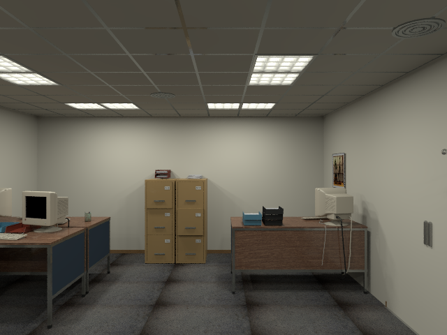
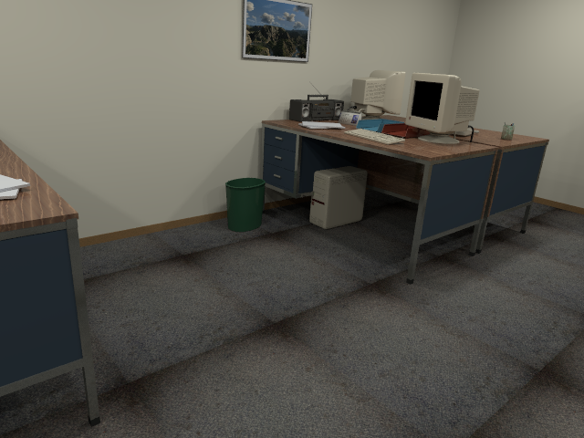
You will be provided with set of artifitially generated image sequence. The sequence contains RGB images with aligned, perfect depth. Format of the images is following:
- color image: RGB with 8 bits per pixel,
- depth image: 16 bit depth values, with scale 5000 per 1m.
| Sample | RGB | Depth |
|---|---|---|
| 100 | 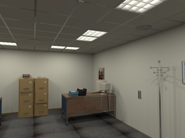 |
 |
Data comes from the ICL NUIM dataset, and the selected sequence is of-kt2.
Original sequence was rendered with 30 frames per second, but for the purpose of this task it was downsampled to 3Hz, i.e. only every 10nth frame was selected.
Feature point view alignment
First step of the algorithm is to calculate the coarse transformation between image pairs. It should be done by detecting and matching features in two images (can be consecutive or spaced by more than one step). Based on those you should calculate 3D coordinates of those points using the depth image and the camera parameters. When two sets of matcihng 3D points are available you have to calculate the transformation between them. After this step you shpuld have a initial camera pose for each frame calculated.
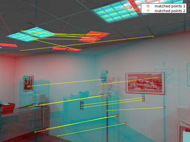
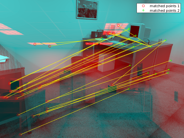
Detecting and matching features
As the exemplary feature detection and matching SURF was selected. After calculating the features for the reference frame (100.png) features for three other frames were calculated and matched. Matches are shown as yellow lines on the picture.
| Sample | Image | Matches |
|---|---|---|
| 100 | |
None (reference image) |
| 110 | 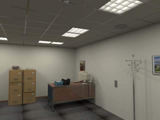 |
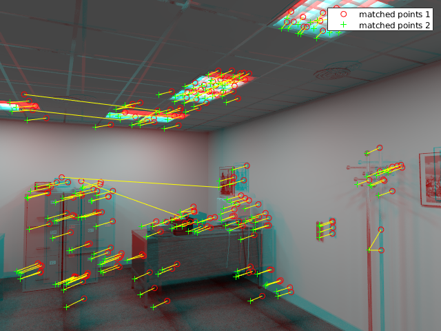 |
| 130 |  |
 |
| 170 |  |
 |
Sample code to detect and match features between two frames is given below. Please remember, that in final solution you should calculate the features for each frame once and store them so that you can use them later without recalculating.
% Read the two images.

I1 = rgb2gray(imread('rgb/0.png'));
I2 = rgb2gray(imread('rgb/10.png'));

% Find the SURF features. MetricThreshold controls the number of detected

% points. To get more points make the threshold lower.

points1 = detectSURFFeatures(I1, 'MetricThreshold', 200);
points2 = detectSURFFeatures(I2, 'MetricThreshold', 200);

% Extract the features.

[f1,vpts1] = extractFeatures(I1, points1);
[f2,vpts2] = extractFeatures(I2, points2);

% Match points and retrieve the locations of matched points.

indexPairs = matchFeatures(f1,f2) ;
matchedPoints1 = vpts1(indexPairs(:,1));
matchedPoints2 = vpts2(indexPairs(:,2));

% Display the matching points. The data still includes several outliers,

% but you can see the effects of rotation and scaling on the display of

% matched features.

figure; showMatchedFeatures(I1,I2,matchedPoints1,matchedPoints2);
legend('matched points 1','matched points 2');
3D coordinates calculation
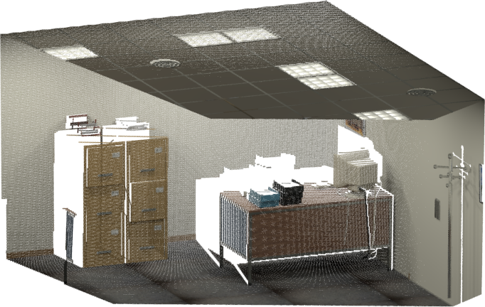
From the feature position in the image (px, py), having the depth value for a given pixel (d) you should calculate real-world coordinates for the interesting feature points. To do this you need camera parameters:
As the data is “perfect”, it has zero distortion. also, the data is dense, so that for every point there is depth value available. Sample full 3D view of selected frame (100.png) looks like this:
Transformation estimation
Based on two sets of matching 3D point sets you have to calculate the initial transformation. Implement the RanSaC algorithm to find the 3D transformation between the points. Please prepare it in a way such that it is possible to change RanSaC parametrs: number of iterations, inliers ratio and reprojection threshold.
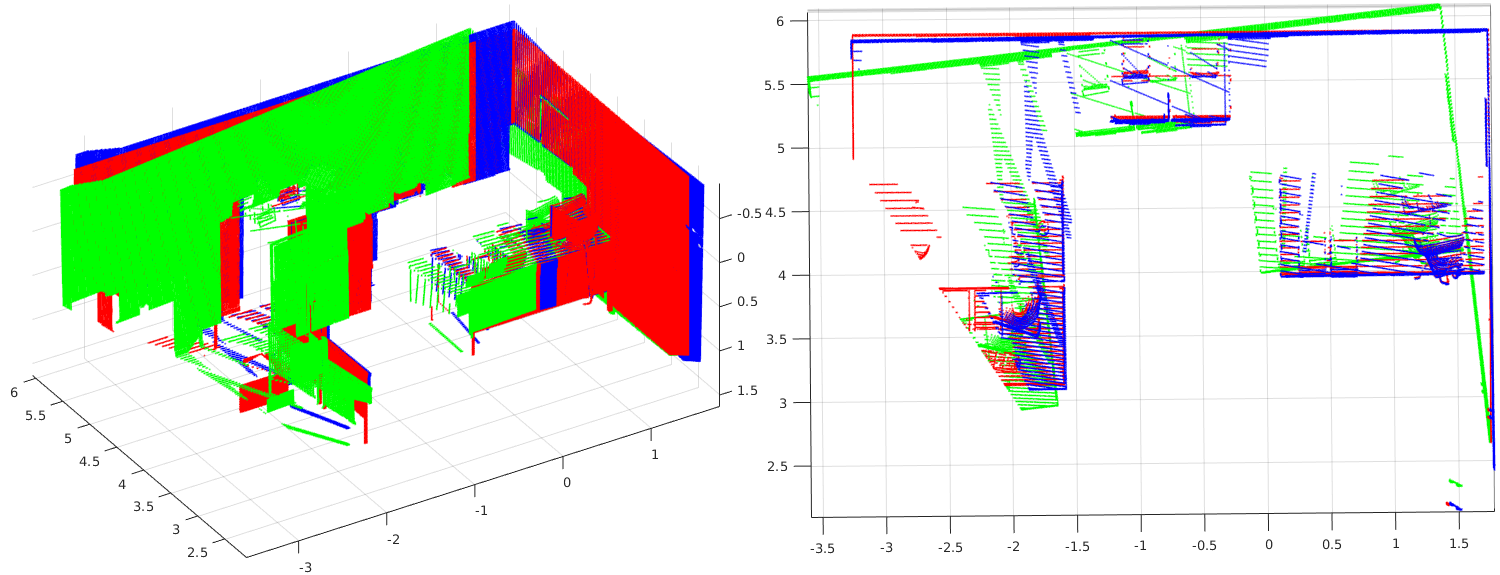
On the image above, red cloud is frame 0 (reference) and green is frame 50. After calculating best initial tranformation green cloud is transformed to the blue, which is more or less overlapping with the red one. For the visualization purpose floor and ceiling were removed.
As a reference for estimating the transformation between subset of points please look at SVD approach by Olga Sorkine-Hornung and Michael Rabinovich from Department of Computer Science, ETH Zurich.
Pairwise transformation refinement
When two pointclouds are initially aligned using RanSaC it is time to further optimise the transformation. Please implement ICP algorithm to align dense pointclouds between the corresponding frames. Same as previously, please allow for changing of ICP parameters in your solution.
Two full XYZ pointclouds should be passed to the ICP algorithm. First one is a reference, sometimes called fixed frame. The second one is going to be aligned with the first one and is called moving. Initial transformation (found in previous step) should be applied, so that the ICP starts close to the final solution.
For this step tou can use pcregistericp function from Matlab. Note, that as an input data should be passed in form of a pointCloud objects.
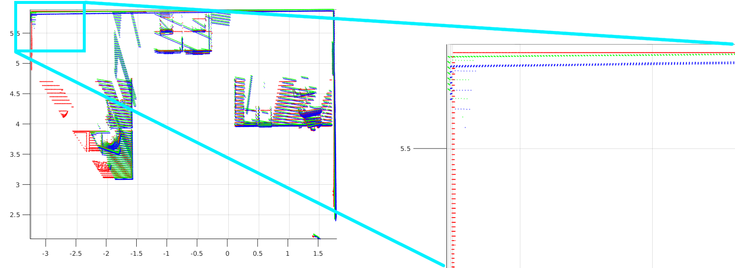
The same pair of frames (0 and 50) before and after ICP refinement. Red is the reference cloud. Blue is the result of RanSaC and green is refined with ICP.
Loop closure
Last step in the project is to detect loops in the data and make global path optimisation. Detect the frames, for which the same part of the view appears again (for example frame 0 and 750):
| 0.png | Matches | 750.png |
|---|---|---|
 |
 |
 |
Final result
After all the steps you should have a list of camera poses for each frame (aligned to the first view). You can display them
using plotCamera function. There is also a reference trajectory for the dataset in the traj.txt file. Format of this
file is: frame_id, tx, ty, tz (position), qx, qy, qz, qw (orientation quaternion). You can load and display this trajectory using
the following script:
% Load reference trajectory from file

traj=load('traj.txt');

% Plot camera poses

figure;
hold on;
axis equal;
numposes = size(traj, 1);
cmap = jet(numposes);
for i=1:numposes
    p=traj(i,:);
    T=p(2:4);      % position

    R=q2r(p(5:8)); % orientation (convert from quaternion)

    cam = plotCamera('Location',T,'Orientation',R,'Opacity',0, 'Size', 0.02, 'Color', cmap(i,:));
end

% Convert [x y z w] quaternion to rotation matrix

function R=q2r(q)
    qx = q(1);
    qy = q(2);
    qz = q(3);
    qw = q(4);

    R = [1 - 2*qy^2 - 2*qz^2   2*qx*qy - 2*qz*qw     2*qx*qz + 2*qy*qw;
         2*qx*qy + 2*qz*qw     1 - 2*qx^2 - 2*qz^2   2*qy*qz - 2*qx*qw;
         2*qx*qz - 2*qy*qw     2*qy*qz + 2*qx*qw     1 - 2*qx^2 - 2*qy^2]';
end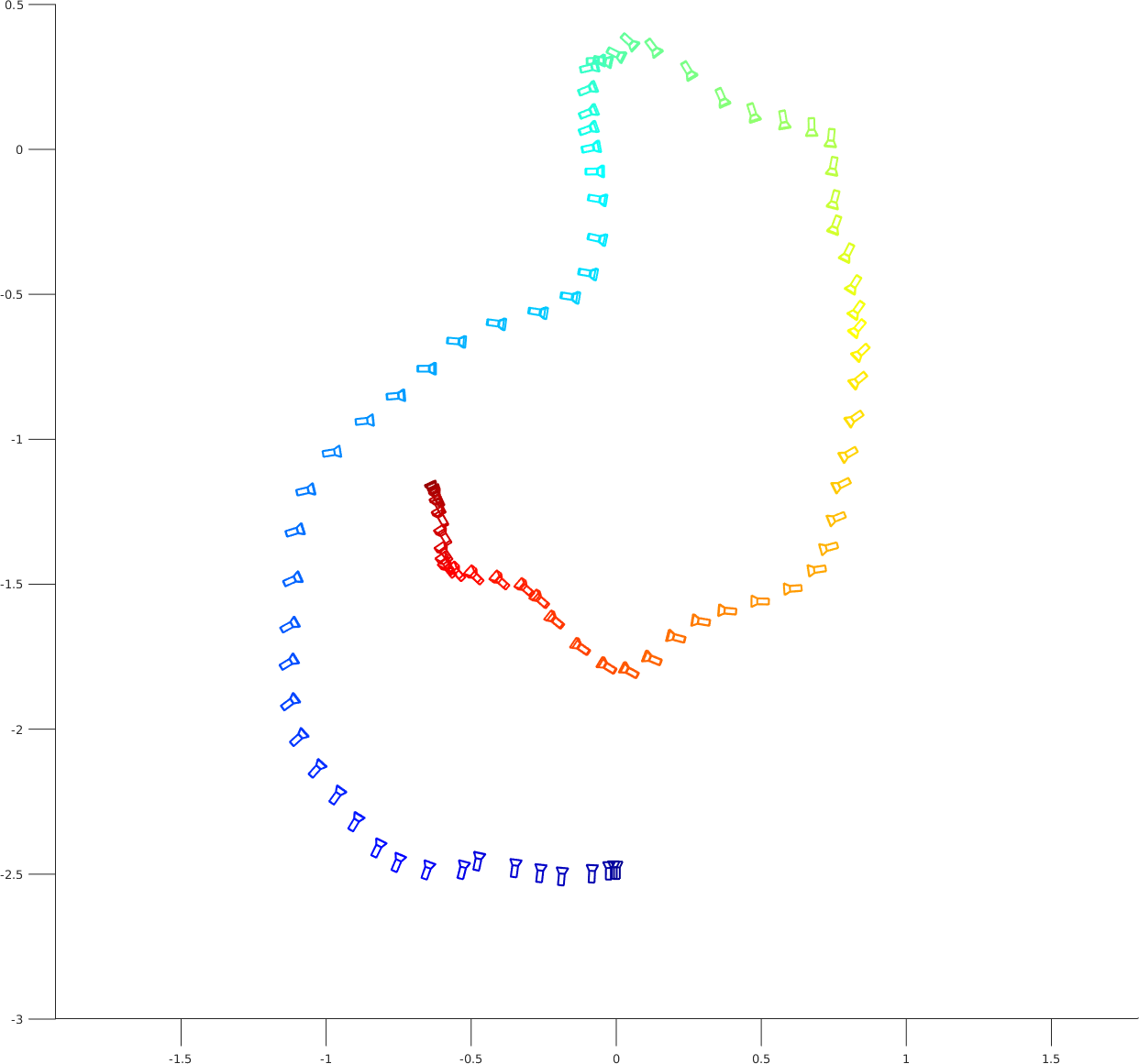
Please compare your result after each step with the reference values. To evaluate your results you cane use RPE and ATE metrics. Tools to calculate them are available on the TUM website.